Updated November 3, 2026. This article covers how Bollinger Bands are calculated and the conditions for interpreting band touches and squeezes. Charts and numbers are illustrative examples built from synthetic data, not measured trading results.
Bollinger Bands are a range whose width follows recent volatility
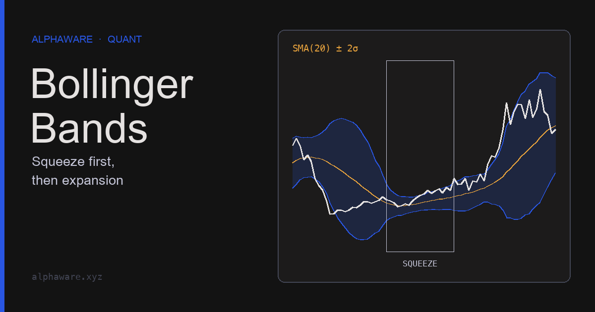
Bollinger Bands were created by John Bollinger in the 1980s. Unlike fixed envelopes drawn a set percentage or distance around a moving average, they set the band width from the standard deviation of recent prices. The bands widen when volatility rises and narrow when it falls.
Bollinger Bands therefore show two things directly: how far the current price is from its recent average in relative terms, and whether recent volatility is high or low compared with the past. They do not show where price will go next.

The defaults are a 20-period average and 2 standard deviations
The default settings Bollinger gives are 20 periods and 2 standard deviations.
| Line | Calculation |
|---|---|
| Middle band | 20-period simple moving average (SMA) |
| Upper band | Middle band + 2 × 20-period standard deviation |
| Lower band | Middle band − 2 × 20-period standard deviation |
Bollinger also defined two related indicators. %B shows where price sits within the bands: 0 at the lower band, 0.5 at the middle band, and 1 at the upper band. Outside the bands it is below 0 or above 1. BandWidth divides the width of the bands by the middle band, so volatility can be compared across periods or securities with different price levels.
%B        = (Price − Lower band) / (Upper band − Lower band)
BandWidth = (Upper band − Lower band) / Middle band
The claim that “about 95% of prices fall inside 2-standard-deviation bands” comes from assuming a normal distribution. Prices do not follow that assumption, and StockCharts ChartSchool, citing Bollinger, says the bands contain roughly 88–89% of price action. Bollinger himself warns against drawing statistical conclusions from the calculation. Platforms may also differ on whether the standard deviation divides by n or n − 1; n − 1 gives slightly wider bands. The code below divides by n.
import numpy as np
import pandas as pd

def bollinger(close, n=20, k=2.0):
    mid = close.rolling(n).mean()
    sd = close.rolling(n).std(ddof=0)      # divide by n; some platforms use n - 1
    upper, lower = mid + k * sd, mid - k * sd
    return pd.DataFrame({
        "mid": mid, "upper": upper, "lower": lower,
        "pct_b": (close - lower) / (upper - lower),
        "bandwidth": (upper - lower) / mid,
    })

rng = np.random.default_rng(7)
quiet = 100 + rng.normal(0, 0.2, 60)
loud = 100 + rng.normal(0, 2.0, 60)
close = pd.Series(np.r_[quiet, loud])
bb = bollinger(close)

# BandWidth follows recent volatility: much narrower in the quiet block.
assert bb["bandwidth"].iloc[40:60].mean() * 5 < bb["bandwidth"].iloc[100:].mean()

# %B is 0 at the lower band, 0.5 at the middle, 1 at the upper band.
row = bb.iloc[-1]
assert np.isclose((row["mid"] - row["lower"]) / (row["upper"] - row["lower"]), 0.5)

# A trending series spends many closes at or above the upper band ("walking the band").
trend = bollinger(pd.Series(100 + np.arange(80.0) + rng.normal(0, 0.3, 80)))
assert (trend["pct_b"].iloc[20:] > 0.9).mean() > 0.5

# The n - 1 convention gives slightly wider bands than the n convention.
s = close.iloc[:20]
assert s.std(ddof=1) > s.std(ddof=0)
A band touch is not a trading signal
“Sell at the upper band, buy at the lower band” is the most common misreading. Bollinger’s rules say otherwise: tags of the bands are just tags, not signals, and closes outside the bands are initially continuation signals, not reversal signals. Many volatility breakout systems rest on that idea.
In a strong uptrend, price can touch the upper band repeatedly as it climbs, which is called walking the bands. The third check in the code above is an example: on a steadily rising synthetic price, %B exceeds 0.9 on most closes. Using upper-band touches as a reason to sell in that situation means trading against the trend. The same happens at the lower band in a downtrend.
To use band touches, define “is the market trending or ranging?” as a separate condition. Choosing that condition after the fact also inflates results, so it has to be tested as a rule fixed in advance.
A squeeze signals contracting volatility, not direction
A state in which the bands have narrowed sharply compared with their own history is called the Squeeze. Bollinger explains that the most popular use of BandWidth is to identify it.
A squeeze does not reveal direction, however. Bollinger Bands alone cannot tell whether price will move up or down after the bands narrow, and the timing of the expansion is not fixed either. To use the squeeze as a rule, set a numeric threshold such as “BandWidth at its lowest in the last N periods,” and fix how the breakout direction is determined.
Widening bands are an observation that volatility has already increased. Band width alone cannot tell whether that marks the start or the end of a trend.
Combine with indicators that carry different information
Bollinger recommends using the bands with other indicators, but choosing indicators that are not directly related to one another. A momentum indicator can complement a volume indicator, while two momentum indicators computed from the same price are no better than one. A lower-band touch together with RSI at or below 30 does not double the reliability, because both reflect the same fact: price has fallen sharply of late.
Bollinger’s W-Bottom, as described by ChartSchool, is an example of a pattern defined in terms of the bands. Turned into a testable rule, it reads:
- The first low forms near or below the lower band.
- Price rebounds toward the middle band.
- The second low is lower than the first but holds inside the lower band (%B above 0).
- Price moves strongly off the second low and breaks above the rebound high.
Defining it this way reduces subjective pattern picking. The sources for this article, however, give no evidence that the rule filters false signals or earns returns. Test it separately, including stop placement, signal count, and costs.
Period and multiplier should move together
20 and 2 are defaults, not answers. Bollinger notes that different markets or purposes may need different values, and recommends raising the standard-deviation multiplier when the period is lengthened and lowering it when the period is shortened. His examples are 2 at 20 periods, 2.1 at 50 periods, and 1.9 at 10 periods. Changing only the period while keeping the multiplier changes how often price closes outside the bands, and so changes what a signal means.
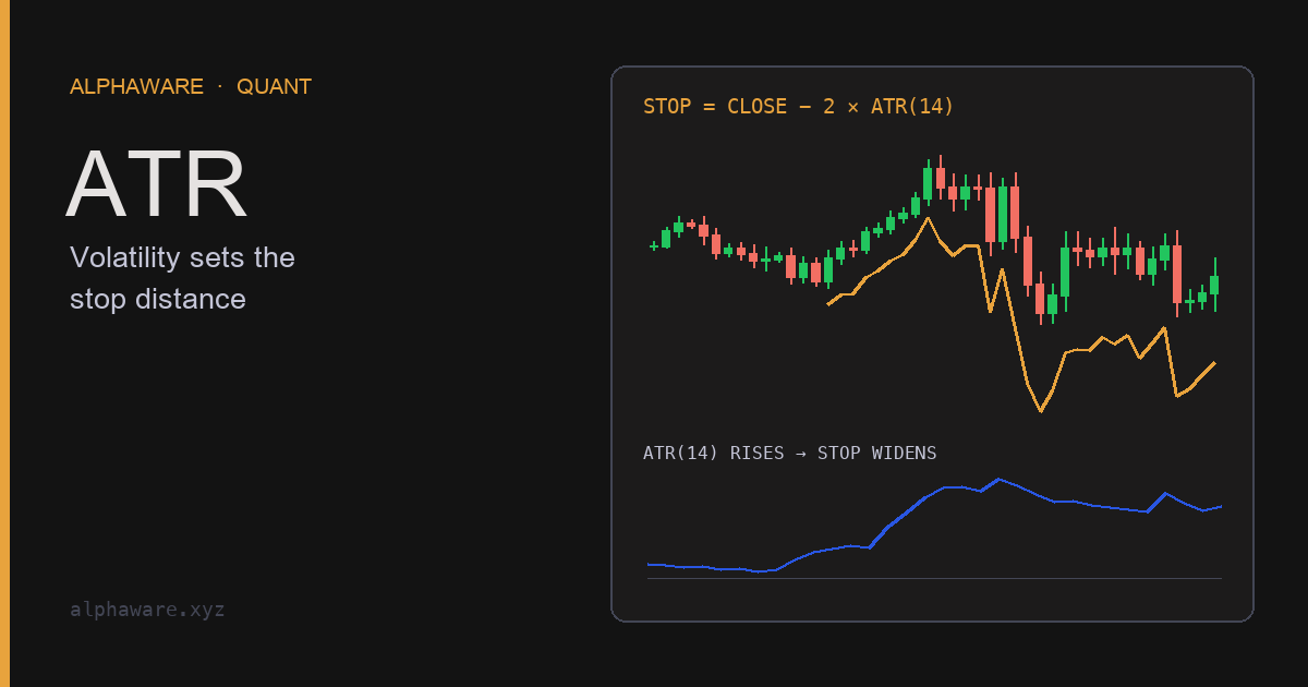
Timeframes need separate treatment too. A stretch that is a squeeze on the daily chart may already be moving one way on the hourly chart. If you tested several combinations of period, multiplier, and timeframe, do not adopt the best one right away; re-check the selection process with the walk-forward methods in Preventing backtest overfitting. Turning volatility into a stop distance in price units is covered in the ATR column.
Sources and scope
- Bollinger Band Rules: the 20/2 defaults, band tags are not signals, closes outside the bands as continuation, combining non-correlated indicators, adjusting the multiplier with the period, BandWidth and the Squeeze.
- StockCharts ChartSchool: Bollinger Bands: formulas, the 88–89% figure, walking the bands, the W-Bottom.
- Wikipedia: Bollinger Bands: development in the 1980s and the explanation, with references, of why the normal-distribution assumption does not hold.
- Park & Irwin (2007), “What Do We Know About the Profitability of Technical Analysis?”: literature review covering data snooping and ex post rule selection in technical trading studies.
- This article explains how Bollinger Bands are calculated and the conditions for interpreting them. It does not claim that rules such as the squeeze or the W-Bottom earn returns, and it is not investment advice.