As of November 2, 2026. This is a data-design article. Dates and values below are hypothetical examples, not actual economic releases or measured investment results.
Chronological splits can still contain future information
You download economic data, sort it by date, train on the earlier section, and validate on the later section. There is no random split. Yet this alone cannot establish that the strategy could have traded at the time: today’s historical file may contain revisions released much later.
A backtest needs two questions answered. Which period does the number describe? Which version could the strategy have known at its decision time? Store only the first date and a row can point to the past while carrying future information.
ALFRED provides vintages for retrieving economic data as available on a historical date, and distinguishes observation dates from the periods during which revisions were current. Today’s best account of the past is a different information set from the one available then. ALFRED download help
Observation, release, and arrival are separate events
Consider a hypothetical monthly index, measured in arbitrary index points.
| Observation period | Available to the system | Value | Version |
|---|---|---|---|
| September | October 5, 13:00 UTC | 100 | Initial release |
| September | November 5, 13:00 UTC | 96 | Revision |
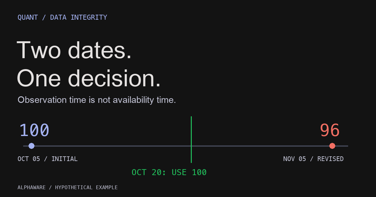
A decision on October 20 can use 100, but cannot use 96. On October 1, neither value is available. Joining either number to September returns merely because the observation month matches introduces information before its release.
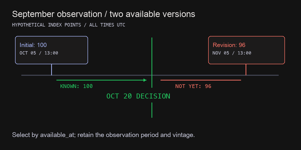
Original conceptual diagram. Values 100 and 96 and all dates are hypothetical. The October 20 decision can use only the initial release.
Release time and arrival time may also differ. A release at 13:00 that becomes usable only after collection and validation at 13:02 should enter an operational replay at the later time. Conversely, do not relabel a file downloaded today as though your system received it ten years ago. Without historical arrival logs, disclose that availability was reconstructed from official release records and an explicit latency assumption.
Append versions instead of overwriting values
The storage unit is a version of an observation, rather than a single number for each date.
| Field | Meaning |
|---|---|
series_id, observation_period |
Series and measured period |
value, unit, adjustment |
Value, units, and seasonal-adjustment basis |
source_released_at |
Verified official release time and zone |
available_at |
Time this version is usable by the strategy |
vintage_id |
Provider’s version identifier |
retrieved_at, source_hash |
Actual download time and raw-file hash |
available_at may be a derived field. Record whether it comes from release time, an assumed delay, or system logs. Keep old versions when revisions arrive so a prior decision remains reproducible.
The ALFRED vintage-date endpoint lists dates when new observations or revisions changed a series. Release dates with unchanged values can be absent. It is therefore not a complete release calendar. FRED vintage-date API
Daily vintages also cannot establish minute-level release timing. An intraday replay needs the original publisher’s timestamps and the delivery path, or a conservative rule that defers uncertain observations to a later decision.
Join on availability before joining on observation period
This example selects versions for one series and one observation period. Apply it separately to each pair in a real dataset, after reconciling units and adjustment conventions.
from datetime import datetime

def dt(text):
    return datetime.fromisoformat(text)

versions = [
    {"available_at": dt("2026-10-05T13:00:00+00:00"), "value": 100},
    {"available_at": dt("2026-11-05T13:00:00+00:00"), "value": 96},
]

def value_asof(rows, decision_at):
    known = [r for r in rows if r["available_at"] <= decision_at]
    if not known:
        return None
    return max(known, key=lambda r: r["available_at"])["value"]

assert value_asof(versions, dt("2026-10-01T00:00:00+00:00")) is None
assert value_asof(versions, dt("2026-10-20T00:00:00+00:00")) == 100
assert value_asof(versions, dt("2026-11-06T00:00:00+00:00")) == 96
Two conflicting values with the same timestamp are ambiguous here. Production code must reject them or define source precedence. The <= boundary assumes that available_at really means usable at that instant. A signal calculated after a closing price is finalized still cannot assume execution at that same close.
This join addresses information availability only. Fitting preprocessing on training data, preventing target-window overlap, and modeling execution timing remain separate obligations. Apply these alongside the validation splits discussed in the overfitting article.
Three invariants to check before returns
First, adding a future revision must not change an earlier decision’s input. Inserting the November revision should leave the October 20 replay unchanged. With identical raw inputs and transformation code, compare selected vintage IDs and feature hashes.
Second, unreleased is not zero. Filling an unreleased value with zero adds an economic assumption. Decide in advance whether to retain missingness, defer the signal, or carry the last known observation for a limited period. If carrying values forward, record their age.
Third, freeze the historical universe too. Vintage-aware macro data do not remove survivorship bias from a universe containing only today’s surviving securities. Adjusted prices, corporate actions, delistings, and membership changes each require their own provider-specific interpretation.
Start with one existing decision rather than reoptimizing a strategy. Reconstruct its input file, selected version, latency assumption, signal time, and execution time. If a timestamp cannot be explained, repair the data contract before interpreting the performance table.
Sources and scope
- ALFRED download help: vintages, observation dates, and real-time validity periods.
- FRED vintage-date API: release dates without changes may be absent.
- The storage schema, delay assumptions, and invariants are implementation proposals in this article. No return improvement or strategy validity is claimed.