Updated November 3, 2026. A method note on the definitions of factor evaluation metrics and the order in which to check them. Numbers in the code come from randomly generated hypothetical panels, not from any real factor or strategy.
IC is a correlation between forecasts and outcomes, not a return
The IC (information coefficient) is the correlation between forecasts and realized outcomes. In Grinold and Kahn’s Active Portfolio Management, IC measures forecasting skill; in practice it is computed as the cross-sectional correlation between assets’ factor values at a point in time and their subsequent returns. Some use Pearson correlation, others a rank (Spearman) correlation, the rank IC, to reduce the influence of outliers. The open-source library Alphalens computes a per-period Spearman rank correlation in factor_information_coefficient.
How IC connects to returns is described by the so-called fundamental law of active management: the information ratio is approximately IC times the square root of the number of independent bets (breadth). Clarke, de Silva, and Thorley (2002) multiplied this by a transfer coefficient, showing that constraints such as no short sales or weight limits reduce how efficiently forecasts are turned into positions.
What the formula makes visible is that with the same IC, results differ when bets are not independent, constraints are tight, or costs are high. The basic formula contains no trading costs. The checks below fill in those blanks.
Look at the distribution of IC across periods, not just its mean
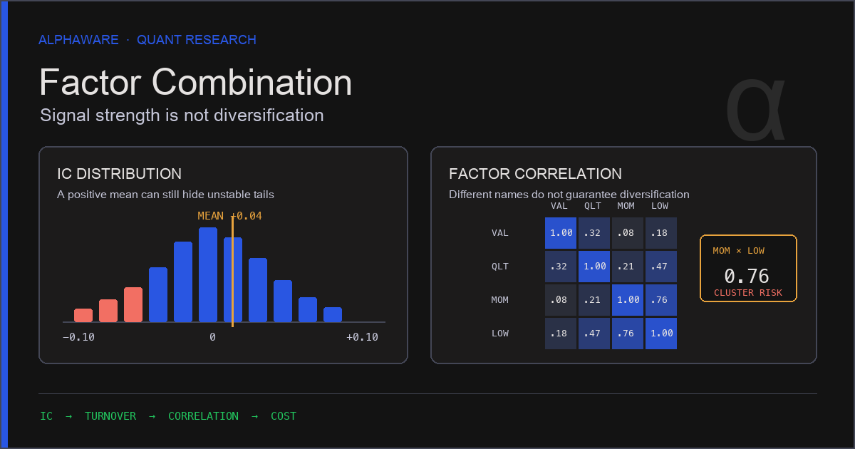
IC is a time series with one value per period. Two factors with the same mean IC should be treated differently if one is steady and the other swings widely. A common summary is the ICIR, the mean of IC divided by its standard deviation.
import numpy as np
import pandas as pd

rng = np.random.default_rng(0)
n_dates, n_assets = 120, 200
dates = pd.date_range("2024-01-05", periods=n_dates, freq="W-FRI")
assets = [f"A{i:03d}" for i in range(n_assets)]

# Hypothetical panel: the factor changes slowly and carries a weak signal for next-period returns
factor = np.zeros((n_dates, n_assets))
factor[0] = rng.normal(size=n_assets)
for t in range(1, n_dates):
    factor[t] = 0.8 * factor[t - 1] + 0.6 * rng.normal(size=n_assets)
noise = rng.normal(size=(n_dates, n_assets))
fwd_ret = 0.05 * factor + noise   # row t: return over the period after t
factor = pd.DataFrame(factor, index=dates, columns=assets)
fwd_ret = pd.DataFrame(fwd_ret, index=dates, columns=assets)

def rank_ic(f, r):
    """Per-date cross-sectional Spearman IC = Pearson correlation of ranks."""
    fr = f.rank(axis=1)
    rr = r.rank(axis=1)
    fr = fr.sub(fr.mean(axis=1), axis=0)
    rr = rr.sub(rr.mean(axis=1), axis=0)
    return (fr * rr).sum(axis=1) / np.sqrt((fr**2).sum(axis=1) * (rr**2).sum(axis=1))

ic = rank_ic(factor, fwd_ret)
icir = ic.mean() / ic.std(ddof=1)
t_stat = icir * np.sqrt(ic.count())   # approximation valid only if per-period ICs are independent

print(f"IC mean {ic.mean():.4f}  IC std {ic.std(ddof=1):.4f}  ICIR {icir:.3f}  t~{t_stat:.2f}")
print(f"share of periods with IC > 0: {(ic > 0).mean():.2f}")

# Rank IC is unaffected by a monotone transform on the same date
assert np.allclose(rank_ic(np.exp(factor), fwd_ret), ic)
assert ic.between(-1, 1).all()
assert ic.mean() > 0
Multiplying ICIR by the square root of the number of periods gives roughly the t-statistic of mean IC. That approximation holds only if the per-period ICs are independent. When the forecast horizon is longer than the rebalancing interval, return windows overlap and the ICs become correlated, so using it as is overstates significance.
We could not confirm a universal threshold above which an ICIR counts as “stable”. The right cut-off depends on asset class, universe size, and rebalancing frequency, so it is better to set and record your own before seeing results. The share of periods with positive IC, the difference between recent and earlier periods, and the average by market regime also show information that a single mean hides.
When rank autocorrelation is low, estimate costs first
If factor ranks change a lot from period to period, the portfolio changes often too. The Alphalens documentation uses the period-to-period autocorrelation of factor ranks, not values, as a turnover measure, noting that if ranks change randomly each period the autocorrelation will be near zero. Ranks are used instead of values to remove systematic shifts in all assets’ factor values.
Applying autocorr() to one long series that concatenates many assets mixes asset boundaries and loses this meaning. Compare cross-sectional ranks date by date.
import numpy as np
import pandas as pd

rng = np.random.default_rng(1)
n_dates, n_assets = 104, 200

def ar_factor(phi):
    """Hypothetical factor panel (dates x assets) with autocorrelation phi."""
    x = np.zeros((n_dates, n_assets))
    x[0] = rng.normal(size=n_assets)
    for t in range(1, n_dates):
        x[t] = phi * x[t - 1] + np.sqrt(1 - phi**2) * rng.normal(size=n_assets)
    return pd.DataFrame(x)

def rank_autocorr(f, lag=1):
    """Cross-sectional rank correlation between dates t and t-lag; ranks remove market-wide shifts."""
    r = f.rank(axis=1)
    return r.corrwith(r.shift(lag), axis=1).dropna()

def top_quintile_turnover(f):
    """One-way turnover per rebalance of an equal-weight long portfolio of the top 20%."""
    w = f.rank(axis=1, pct=True).gt(0.8).astype(float)
    w = w.div(w.sum(axis=1), axis=0)
    return 0.5 * w.diff().abs().sum(axis=1).iloc[1:]

def annual_cost(turnover, cost_rate, periods_per_year):
    """Annual cost ~ rebalances per year x turnover per rebalance x cost per unit traded."""
    return periods_per_year * turnover.mean() * cost_rate

slow, fast = ar_factor(0.95), ar_factor(0.30)
for name, f in [("slow", slow), ("fast", fast)]:
    to = top_quintile_turnover(f)
    print(f"{name}: rank autocorr {rank_autocorr(f).mean():.2f}, "
          f"turnover {to.mean():.2f}, annual cost {annual_cost(to, 0.001, 52):.2%}")

assert rank_autocorr(slow).mean() > rank_autocorr(fast).mean()
assert top_quintile_turnover(slow).mean() < top_quintile_turnover(fast).mean()
# 5.2% a year only if the whole portfolio is replaced every week (turnover 1.0) at 0.1% cost
assert np.isclose(annual_cost(pd.Series([1.0]), 0.001, 52), 0.052)
The rule of thumb “0.1% cost with weekly rebalancing means about 5% a year” holds only if the entire portfolio is replaced every week. In this hypothetical example, the factor with rank autocorrelation 0.95 had turnover of about 18% per rebalance and the one with 0.30 about 66%, so annual cost estimates at the same cost rate differed several-fold. Real costs depend on spreads, market impact, commissions, taxes, and borrow costs, so check how sensitive the result is by varying the cost rate.
Adding similar factors enlarges the same bet
Combining several factors does not add independent bets if they measure the same information. Breadth in the fundamental law counts independent bets, so adding highly correlated factors is closer to increasing the weight of one signal than to diversifying. Momentum factors cut from the same price history at different lengths, for example, share calculation windows and are likely to be correlated. The actual level has to be checked in the data.
import numpy as np
import pandas as pd

rng = np.random.default_rng(2)
n_dates, n_assets = 104, 200

def xs_rank_corr(a, b):
    """Average of per-date cross-sectional rank correlations between two factors."""
    return a.rank(axis=1).corrwith(b.rank(axis=1), axis=1).mean()

base = pd.DataFrame(rng.normal(size=(n_dates, n_assets)))
near_copy = base + 0.3 * rng.normal(size=base.shape)      # remeasures almost the same information
other = pd.DataFrame(rng.normal(size=(n_dates, n_assets)))  # separate information

c_dup, c_ind = xs_rank_corr(base, near_copy), xs_rank_corr(base, other)
print(f"near-copy corr {c_dup:.2f}, independent corr {c_ind:.2f}")
assert c_dup > 0.8 and abs(c_ind) < 0.05

# IC by horizon: rank correlation between factor(t) and the one-period return k periods later
phi = 0.7
f = np.zeros((n_dates, n_assets))
f[0] = rng.normal(size=n_assets)
for t in range(1, n_dates):
    f[t] = phi * f[t - 1] + np.sqrt(1 - phi**2) * rng.normal(size=n_assets)
f = pd.DataFrame(f)
ret = 0.1 * f + rng.normal(size=f.shape)   # row t: return from t to t+1

ic_by_lag = {k: xs_rank_corr(f, ret.shift(-k)) for k in [0, 1, 2, 4, 8]}
for k, v in ic_by_lag.items():
    print(f"lag {k}: IC {v:.4f}")
assert ic_by_lag[0] > ic_by_lag[2] > ic_by_lag[8]
Rather than pooling all periods into one correlation matrix, computing per-date cross-sectional correlations as above and looking at their mean and variation better matches what combining factors means. When you find a highly correlated pair, options include dropping one, orthogonalizing by regression, or grouping them into principal components. Where to draw the line depends on criteria set in advance and on how the combined IC and turnover change.
Use IC by horizon to choose candidate rebalancing frequencies
The second part of the code above computes IC while increasing the lag between when the factor is measured and the return window. How quickly IC falls as the lag grows is the lifespan of the factor’s predictive power. In the hypothetical example, IC was about 0.10 at lag 0 and near zero at lag 8.
This curve gives candidates for the rebalancing frequency. If IC decays slowly, you can test rebalancing less often to save costs; if it decays quickly, frequent rebalancing is needed to use the signal, and the cost estimate in the previous section matters more. The final choice comes from comparing net-of-cost results across frequencies.
When comparing IC over cumulative return windows (for example 1, 5, and 21 days), also keep in mind that longer windows overlap more, which increases autocorrelation in the IC series.
Order of checks before adding a factor
This sequence assumes the thresholds are set before seeing the results.
- Overlap with existing factors: check the mean and variation of per-date cross-sectional rank correlations. If high, decide whether to drop, orthogonalize, or change how factors are combined.
- Distribution of IC: look at mean, standard deviation, ICIR, share of positive periods, and differences across sub-periods. Do not take the t-statistic at face value when return windows overlap.
- Rank autocorrelation and turnover: compute turnover per rebalance with the portfolio rule you would actually use, and estimate annual cost while varying the cost rate.
- IC by horizon: use the rate of decay to pick candidate rebalancing frequencies.
- Net-of-cost validation: for each candidate frequency, run a chronological validation that includes costs and constraints. Split methods are covered in the overfitting checks article.
Sources and scope
- Clarke, de Silva, Thorley (2002), Portfolio Constraints and the Fundamental Law of Active Management, Financial Analysts Journal 58(5): generalizes Grinold’s fundamental law with a transfer coefficient. Definitions of IC and breadth follow Grinold & Kahn, Active Portfolio Management (2nd ed., McGraw-Hill, 2000).
- Alphalens API reference: definitions of
factor_information_coefficient(per-period Spearman IC) andfactor_rank_autocorrelation(rank autocorrelation as a turnover measure). - This article gives no threshold values for ICIR, turnover, or cost. It describes a factor evaluation procedure and does not claim that any factor or combination method produces excess returns.